Maximizing Revenue With Machine Learning for Retail Pricing

Summary

Mosaic helped a nationwide retailer model the price elasticity of demand across their product catalog, empowering them to optimize prices and maximize SKU revenue.

Introduction

For retailers across the nation, predicting the effect that a change in sales price will have on demand is vital to optimizing prices and maximizing sales revenue. Without a reliable model, retailers rely on gut feel and Excel-based tools to answer critical questions such as:

How much will sales increase if I drop my price by X% to get inventory out the door?

How much will sales decrease if I increase my price by X% to avoid stock-outs?

According to McKinsey, effectively and profitably linking pricing and promotions together using machine learning for retail pricing can increase revenue and profiles by three to five percentage points overall. In addition, companies that efficiently implement this approach often achieve improved customer satisfaction and loyalty.

Mosaic helped a nationwide retailer answer these questions across their product catalog, a critical first step for their pricing team to optimize and standardize pricing across several thousand SKUs. The retailer was struggling with finding the right processes and tools to guide decisions on pricing. Mosaic matched the proper analytics tool and technique with their specific use case, delivering actionable predictive and prescriptive analytics regardless of the company’s level of analytics maturity.

At every phase during the project, Mosaic acted as a true partner, collaborating effectively with the retailer to make sense of the observations uncovered in the data and the implications that certain estimates might have on the business. Mosaic interchanged data scientists with the team as requirements shifted, helping the firm set profitable prices while maintaining a consistent customer experience. Mosaic was critical in enabling the retailer to design & deploy machine learning for retail pricing.

Price Elasticity of Demand

The key economic law underpinning this modeling effort is the price elasticity of demand. This is a measurement of the estimated change in demand in relation to a change in price. If the price changes by X%, the elasticity coefficient is the percentage by which we expect demand to change as a response. Here is how the price elasticity of demand is expressed mathematically:

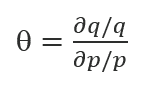
Where the elasticity coefficient θ is equal to the change in demand q divided by the change in price p. For example:

• If price increases by 20% and demand drops by 10%, elasticity coefficient is -10/20 = -0.50
• If price decreases by 20% and demand increases by 10%, elasticity is also -0.50

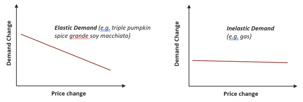
Economists assume that elasticity is linear and that the coefficient is constant across all price changes. Elasticity coefficients are typically negative values and will vary depending on the product in question. Some products are more elastic than others. For example, a grande triple pumpkin spice soy macchiato is more elastic than gas because when inflation goes up, gas is more essential.

Examples of factors that affect the price elasticity of demand for a product are:

• Necessity: The more necessary a product is, the lower the elasticity. This implies that even large increases in price will result in small decreases in demand.
• Substitutability: Elasticity will be higher if more substitutes are available. For example, large increases in price will result in large decreases in demand because consumers have other options.
• Brand loyalty: Where consumers are attached to a particular brand, elasticity tends to be lower because consumers are still willing to buy a product even if the price increases.
• Duration: If a higher price holds for a long time, consumers tend to accept the new price, resulting in less elastic demand.
• Income effect: The higher the percentage of a consumer’s income relative to a product’s price, the higher the elasticity typically is. The more negligible the price change is relative to income, the less elastic it is.
• Breadth of definition: The broader the definition of a good or service, the lower the elasticity tends to be. For example, food in general is not very elastic, while specific types of food may be more elastic (e.g. seafood) because consumers have other options.
• Addictiveness: Goods that are more addictive tend to be less elastic. This relates to necessity because consumers who are addicted to cigarettes treat them as necessary.
• Payer: When the consumer does not directly pay for a good (e.g. corporate expense accounts), demand is typically less elastic. For example, a price hike at a high-end restaurant will be negligible if the consumer pays for the meal with a company card.

Price Elasticity of Demand Modeling

Mosaic engaged with a nationwide retailer to deliver models using machine learning for retail pricing that would determine price elasticity of demand across their product catalog. Here we describe the high-level approach taken to develop these prototype models.

Transaction Data Pre-Processing

We began with the pre-processing of historical transaction data. Because the data is in a raw state, significant effort was made upfront to get the data into a state where valid observations of price changes and subsequent demand changes could be observed. Although there are several hundred million transactions over several years, we care most about the transactions that occurred before and after a price change event.

At a high level, Mosaic implemented the following steps to wrangle raw transaction data into valid price and demand change observations.

Price change observations were taken at the SKU level, while elasticities were later estimated at higher product category levels because individual SKUs rarely have enough observations to model out properly.

Price change events were then flagged for each SKU. These events ultimately became individual samples that were fed into the model. Demand (sales) were aggregated for each SKU n days before and after each price change. Then a raw demand change was calculated using the before and after SKU demand.

Because the raw demand change may include other factors extraneous to the actual price change, Mosaic calculated a baseline demand change that can be used to adjust the demand change to reflect only the effect of the price change on demand. Examples of extraneous factors include:

• Normal seasonal demand changes (e.g., significant increase in demand during the Christmas season).
• Marketing campaigns focused on advertising certain types of products.
• Product placement changes in the store or website that are geared toward increasing sales.

The baseline demand change was observed using a broader category of products to which the individual SKU belonged. For example, if the SKU in question is a T-shirt, we look at the broad shift in demand for clothing in general and use it to account for broad shifts in demand that may be bound up in the observed demand change for the T-shirt.

SKUs that are short on inventory during the observation window were excluded, as these observations may have steep increases or drops in demand that are due to inventory levels. Additional pre-processing steps may be taken for different retailers depending on the nature of the business and the transaction data.

An example of processed data ready for modeling is shown below:

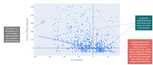
Machine Learning for Retail Pricing Visualization

Linear Mixed Effects Modeling

The elasticity of a product can also be viewed as the coefficient of price change when using price change to predict demand change in the following regression equation:

Δ demand = θ Δ price

Where Δ demand is the change in demand, θ is the elasticity coefficient, and Δ price is the change in price. Note that we do not include an intercept (b) because we assume that no change in price would result in no change in demand.

Next, because of the hierarchical nature of the retailer’s product catalog, Mosaic took a Linear Mixed Effects approach to estimate the elasticity coefficients for each level of the product hierarchy. Linear Mixed Effects modeling allows for coefficients to be estimated across all samples (e.g., an entire department) and individual coefficients to be estimated for different subgroups within the larger group. This works well for nested groups that are common in retail product catalogs. The generalized linear mixed effects model can be described as follows:

y = βX +uX + ε

Where:

• y is the dependent variable (e.g., demand change)
• β are the fixed effect coefficient(s) applied to each dependent variable (X, which in this case is only price change). An example of a fixed effect would be the coefficient on the entire department that applies to all observations.
• u are random effect coefficients that are also applied to X An example of a random effect would be individual coefficients that only apply to observations of a specific subgroup within the department.
• ε are random error terms with mean = 0

An example of the estimate coefficients out of a linear mixed effects model is given below:

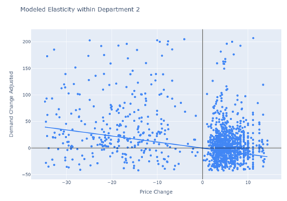
The blue line represents the estimated resulting percentage change in demand following a percentage change in price. The coefficient governing that line is the elasticity coefficient and is applied to all products within the department.

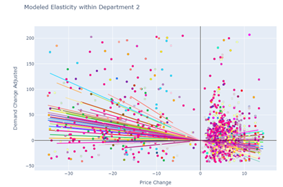
Underneath the department, there are several subgroups of products. An individual coefficient is estimated for each subgroup as well. This allows the pricing team to leverage multiple elasticity estimates to make broad and narrow pricing decisions. Although elasticity estimates are often desired as close to the SKU level as possible, this approach enables the pricing team to obtain a good elasticity estimate from a higher level of the product hierarchy when not enough samples are available for an individual SKU.

Conclusion

In partnering with Mosaic’s hands-on, expert team of data scientists, the retailer was able to achieve reliable estimates of how their pricing decisions will impact demand, empowering them to begin optimizing and standardizing pricing across the business to maximize returns. The models also helped the retailer save dozens of hours in manpower by trading outdated, legacy tools for powerful, accurate results.

Machine learning techniques produce accurate predictive models of demand-price elasticity, which can help retailers stay competitive and maximize profit gains.  Historical transaction data from before and after a price change event can act as a starting point for the modeling, lending insight into price changes and subsequent demand changes. Using this data, machine learning for retail pricing applications can calculate price elasticity, measuring how demand will fluctuate due to shifts in pricing strategy.