Data Science Design Pattern #3: Handling Null Values

Why Handling Null Values Matters

Most data science algorithms do not tolerate nulls (missing values). So, one must do something to eliminate them, before or while analyzing a data set. How does one go about handling null values?

Description

There are many techniques for handling null values. Which techniques are appropriate for a given variable can depend strongly on the algorithms you intend to use, as well as statistical patterns in the raw data—in particular, the missing values’ missingness, the randomness of the locations of the missing values.[i]  Moreover, different techniques may be appropriate for different variables, in a given data set.  Sometimes it is useful to apply several techniques to a single variable.  Finally, note that corrupt values are generally treated as nulls.

Classes of missingness.  The locations of the missing values can fall into one of three cases:

Missing completely at random (MCAR) values are randomly drawn from the sample, independent of other variables.

Missing at random (MAR) variables are randomly distributed, conditional on other variables.

Missing not at random (MNAR) variables’ missingness still depends on the missing values, even conditional on other variables.

Classes of techniques.  Techniques for handling nulls fall into four classes (in increasing order of sophistication):  null deletion, naïve central-value estimators, other algorithm-independent functions, and algorithm-specific functions.  All but the first replace a null with a surrogate value computed by some means.

Null deletion.  Here one merely deletes null values, or the records containing them, from the original data set.  In case-wise deletion one deletes all records containing null values.  In pairwise deletion one only deletes records containing null values of variables used by a specific analysis.

Naïve surrogates.  The easiest surrogate values are unconditioned central values—mean, median, or mode.[ii]  (Random and constant values are alternatives.)

Algorithm-independent surrogates.  A more sophisticated way to compute a surrogate value is to use a predictive algorithm to estimate the missing value, independent of the algorithms you might use later to analyze the data.  We have already seen that smoothing is one way to handle missing data.  It applies, in particular, when insufficient history has accrued to distribute mass over a source variable’s set of possible values; we then redistribute probability mass from observed to missing values.  (See design pattern #2 for details.)  Other approaches include variants of regression, Bayesian conditioning, and maximum likelihood.  When the nulls are not missing at random, it may be necessary to account for the non-randomness in the predictive model used to compute surrogates.

Algorithm-specific surrogates.  Some analytical algorithms compute a context-appropriate surrogate value while analyzing the data.  For example, some random-forest algorithms have multiple runtime strategies for replacing nulls (in training and test sets) with values that depend on the type of variable and where in the forest the algorithm uses the variable.[iii]  (One can also use random forests to generate algorithm-independent surrogates.)

How it Works

The third approach is the interesting case.  (The other approaches are trivial to execute.  In particular, the fourth approach is generally built into the implementation of the analytical algorithm, so one can treat the algorithm as a “black box.”)  The general procedure is to use the non-null sample values to build a model that predicts a variable having missing values, and then substitute the model’s predictions for each missing value of that variable.

Techniques such as multiple imputation[iv] (MI) use sampling techniques or introduce noise to account for the extra variance introduced by replacing missing values.  MI is among the state of the art algorithm-independent techniques.  MI implementations exist for regression, time series, categorical data, etc.[v]  The general MI algorithm has three steps:

1. Repeatedly (m times) impute values to each missing variable, yielding m complete data sets.
2. Analyze the m data sets to produce m sets of parameter estimates.
3. Pool the m estimates into a single set of parameter means, variances, and confidence intervals.

When to Use It

Null deletion.  You are free to delete records containing nulls when two conditions apply:

1. You are confident that the null values are MCAR.
2. The data are sufficiently abundant, or the records containing nulls are sufficiently sparse, so that your sample size will not change substantially as a result of deleting those records.

In this case deleting nulls is a fast way to get past them.  Otherwise, null deletion distorts the source data’s distribution, causes detrimental data loss, or both.

Naïve surrogates.  Central-value surrogates are safest when

1. You are confident that the sample comes from a unimodal, symmetric distribution that has a well-defined mean and variance.[vi]
2. The data is abundant.
3. The number of null values is small.
4. The distribution has a small variance (so that most of its values are near the mean).

In such cases substituting a central value should have a small effect on the analysis.  When in doubt, you may wish to perform a sensitivity analysis, to check that the choice of surrogate value does not substantially alter the results.

Algorithm-independent vs. algorithm-specific surrogates.  We encourage you to use algorithm-specific techniques when they exist, and otherwise to use robust algorithm-independent techniques such as MI.  Either approach generally improves substantially on the naïve and null-deletion alternatives.

Example

Figure 1 below contains R code that does the following:

1. Construct a sample of body weights for a large population of both males and females between the ages of 10 and 90, modeled as a function of age and gender, with some Gaussian noise added to the weights.
2. Deletes 10% of the weight values.
3. Imputes several naïve estimators to the missing values.
4. Uses a linear-regression MI algorithm in the R Hmisc library to estimate the missing values.
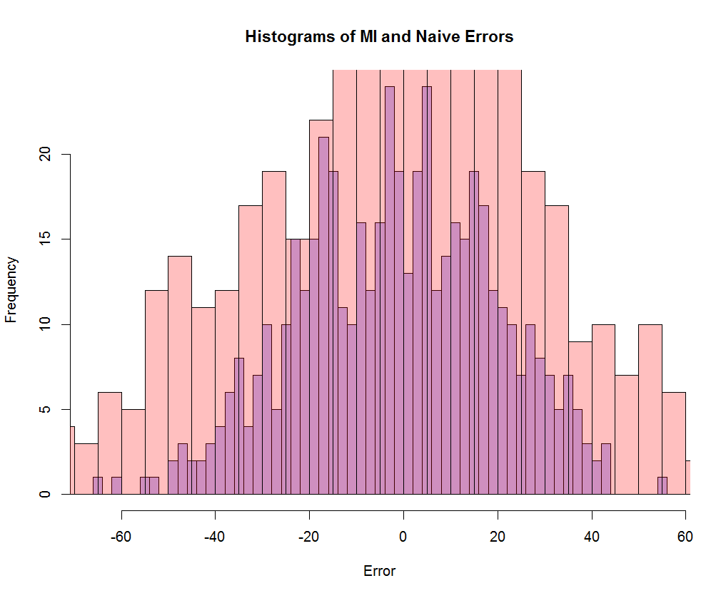
5. Compares the naïve (mean imputation) and MI results.

The standard deviations of the errors are 29.6 and 20.9, respectively, indicating significant improvement over the naïve approach.  (Further improvement might be possible if one allowed Hmisc’s aregImpute() function to fit a nonlinear model.)

library(Hmisc)
n <- 5000
m <- n/10 

# Generate a random sample of individuals having age, gender, and weight.
# (Gender is 1 for males, so males can be heavier on average.)
# Weight ~ age + gender + Gaussian noise 

sampleData <- data.frame(
  age = sort(sample(10:90, n, replace = TRUE)),
  gender = sample(0:1, n, replace = TRUE)
)
sampleData$weight <-
  (75 + (10 * sampleData$gender)) * log10(sampleData$age) +
  rnorm(n, mean = 0, sd = 20) 

# Make a copy of the weight data, for later reference.

sampleDataWeight <- sampleData$weight

# Make m weight values go away, choosing the locations MCAR.

sampleData$weight[sample(1:n, m, replace = FALSE)] <- NA

# naive surrogates:  impute mean, median, random, or fixed value
# (we can do this because the data is MCAR by construction)

sampleData$mean_imputed_weight <- with(sampleData, impute(weight, mean))
sampleData$median_imputed_weight <- with(sampleData, impute(weight, median))
sampleData$random_imputed_weight <- with(sampleData, impute(weight, ‘random’))
sampleData$fixed_imputed_weight <- with(sampleData, impute(weight, 144)) 

# multiple imputation using a full Bayesian predictive distribution
# and a linear-regression model 

miModel <- aregImpute(
   ~weight + age + gender,
   data = sampleData,
   n.impute = 10,
   type = “regression”
)

# compare MI and naive (impute mean to all NAs) errors 

sampleData$finalWeight[1:n] <- sampleData$weight
sampleData$finalWeight[as.integer(dimnames(miModel$imputed$weight)[[1]])] <-
   rowMeans(miModel$imputed$weight)
sampleDataError <-
   sampleDataWeight[as.integer(dimnames(miModel$imputed$weight)[[1]])] –

sampleData$finalWeight[as.integer(dimnames(miModel$imputed$weight)[[1]])]
naiveError <-
   sampleDataWeight[as.integer(dimnames(miModel$imputed$weight)[[1]])] –
   mean(sampleData$weight, na.rm = TRUE)

describe(sampleDataError)
describe(naiveError) 

sd(sampleDataError)
sd(naiveError)

sampleErrorHistogram <- hist(sampleDataError, breaks=m/10)
naiveErrorHistogram <- hist(naiveError, breaks=m/10)
plot(
   sampleErrorHistogram,
   col=rgb(0,0,1,1/4),
   main = “Histograms of MI and Naive Errors”,
   xlab = “Error”,
   ylab = “Frequency”
)
plot(
   naiveErrorHistogram,
   col=rgb(1,0,0,1/4),
   add=TRUE, 
   main = “Histograms of MI and Naive Errors”,
   xlab = “Error”,
   ylab = “Frequency”
)

Figure 1:  Sample R Code for Naïve and MI Surrogate Values

Figure 2 overlays the naïve and MI error histograms.  (The narrower histogram is the MI error, indicating that MI improves on the naïve imputation’s estimation error.)

See Stekhoven (2011)[vii] for examples of nonparametric null imputation using a random-forest algorithm (in R’s missForest package).

[i] R.J.A. Little & D.B. Rubin, Statistical Analysis with Missing Data (Wily, 1987); P.D. Allison, Missing Data (Sage, 2001); D.C. Howell, “The Analysis of Missing Data,” Handbook of Social Science Methodology (Sage, 2007); and A.N. Barladi & C.K. Enders, “An Introduction to Modern Missing Data Analyses,” Journal of School Psychology 48 (2010), pp. 5-37.

[ii] These and similar techniques are now considered dated.  There are many resources online, contributed by the academic community for handling null values:  http://www.uvm.edu/~dhowell/StatPages/More_Stuff/Missing_Data/Missing.html and http://www.uvm.edu/~dhowell/StatPages/More_Stuff/Missing_Data/Missing-Part-Two.html,
http://www.utexas.edu/cola/centers/prc/_files/cs/Missing-Data.pdf,
http://www.stat.columbia.edu/~gelman/arm/missing.pdf (visited March 2, 2014).

[iii] For example, see http://www.stat.berkeley.edu/~breiman/RandomForests/cc_home.htm#missing1 and http://cran.r-project.org/web/packages/missForest/missForest.pdf (visited March 2, 2014).

[iv] Multiple imputation averages estimated parameters over multiple runs of the estimation model, each of which uses different imputed values, to build the final estimation model, for handling null values.  See Stef Van Buuren, Flexible Imputation of Missing Data (Chapman & Hall, 2012).

[v] Van Buuren lists nearly 20 related R libraries alone at http://www.stefvanbuuren.nl/mi/Software.html (visited March 2, 2014).

[vi] Several important classes of distributions do not have central values.  The uniform distribution is a trivial example.  Lévy-stable distributions with α  ≤ 1 don’t have means.  See John P. Nolan, Stable Distributions:  Models for Heavy-Tailed Data (Birkhauser, 2013), available in part at http://academic2.american.edu/~jpnolan/stable/chap1.pdf (visited March 2, 2014).  The Cauchy distribution is one such heavy-tailed distribution.  Its mean and variance are undefined.  See http://en.wikipedia.org/wiki/Cauchy_distribution (visited March 2, 2014).  Lévy-stable distributions occur in financial modeling, physics, and communications systems.  Where a variable is the sum of many small terms, e.g. the price of a stock or the noise in a communications signal, it may have a stable distribution.

[vii] http://stat.ethz.ch/education/semesters/ss2012/ams/paper/missForest_1.2.pdf (visited March 2, 2014).