Proper customer segmentation is crucial to drive effective marketing strategies, predict demand and optimize pricing. At its heart, segmentation is about grouping similar customers to describe and predict their purchasing behavior. The key question here is what such grouping must be based on. This is where geospatial data analysis comes in.
One possibility is to select the grouping a priori and then ask about purchasing habits, for example, when we segment customers based on demographics. This approach is useful to characterize behaviors using groups we already have a concept for, like age segments. However, it may be challenging sometimes to decide the best way to split a dimension like age, e.g., how many age groups do we want? What ages should be included in each bin?
Another possibility is to let the purchase data speak for itself and use machine learning to uncover potential clusters. This alternative was discussed in a previous blog entry titled Using Transaction Data for Optimal Customer Segmentation Analysis.
In this article, Mosaic highlights how geography can inform segmentation efforts through spatial analysis, which leverages spatial data, location data, satellite and aerial imagery, or any other form of geographic information to build machine learning models and gather usable insights for customer segmentation. Combining geospatial data with machine learning presents ample opportunity to leverage structured information to inform business decisions.
Geography Based Analytics
The most common way of using geospatial data analysis in customer segmentation is to use spatial divisions such as cities or postal code regions as the basis for different aggregations and stats. Calculations such as click-through and close rates by ZIP code are typical indicators to drive customer acquisition investments and marketing campaigns. Geography-related aspects are also crucial for business location decisions.
One important consideration that must not be neglected is the granularity of the spatial divisions used to segment customers. Indeed, we must be aware that, in general, one limitation of customer segmentation analytics is that we characterize all customers within each segment by a unique vector of attributes.
In other words, we treat everybody in a segment as if they behave the same way, thus losing track of all the intra-segment heterogeneity. While this may be good enough if the low variance, we will likely discover multiple patterns in highly heterogeneous segments. This is particularly noticeable when we use divisions such as postal codes, county lines, or larger regions due to various reasons such as:
- Uneven population density
- Spatial divisions (postal code area, county, state) vary significantly in area
- Seasonality in transportation patterns at daily, weekly, monthly, and annual levels
- Each region has differences in access to services and business, household incomes, purchase power, crime rates, etc..
What do we know about our customers?
The first question to pay attention to is what customer-related spatial information is available. For example, many businesses resort to wide-net marketing strategies driven by proximity to generate leads. Still, lack of mechanisms to track the actual geographic origin of their customers, thus missing the opportunity to identify where the marketing campaign has more resonance.
By contrast, other businesses employ different ways of personalizing their promotions and interactions with current and potential clients, thereby making it possible to know the point of origin of each customer. Strategies such as personalized mail or smartphone apps are ways to collect data about geographic displacements.
Spatial Analysis
Knowing where people work and live and where they go shopping, for example, may be useful for conducting a geospatial data analysis and calculating interesting indicators like market penetration at the postal code level. Indeed, a business located in a particular ZIP code area may be interested in knowing how many customers live in each one of the surrounding zones.
However, as we mentioned before, postal code areas can vary significantly in surface, the density of people, and businesses. Also, some geographic characteristics like landscape, among other things, make people prefer certain routes.
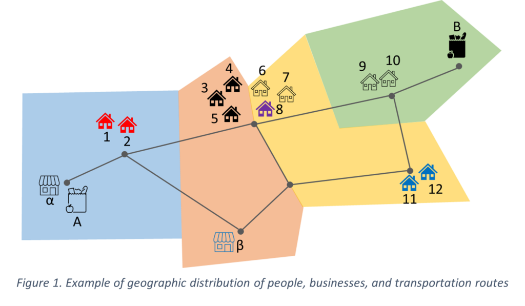
To illustrate the alternative ways of exploiting geographic information, consider the example shown in Fig. 1. Four postal codes areas are highlighted by diverse colors, each of which contains houses (1 to 12), along with supermarkets (A, B) of the same chain, two competing businesses (α, β) and are communicated by a transportation network. The distribution of visits to each commercial destination is shown in the next table.
| Origin | Destination | ||||
| Zip | Origin | A | B | α | β |
| Blue | 1 | 100% | 0% | 100% | 0% |
| 2 | 100% | 0% | 100% | 0% | |
| Orange | 3 | 100% | 0% | 100% | 0% |
| 4 | 35% | 65% | 35% | 65% | |
| 5 | 60% | 40% | 5% | 95% | |
| Yellow | 6 | 10% | 90% | 0% | 100% |
| 7 | 1% | 99% | 3% | 97% | |
| 8 | 100% | 0% | 100% | 0% | |
| 11 | 0% | 100% | 0% | 100% | |
| 12 | 0% | 100% | 0% | 100% | |
| Green | 9 | 0% | 100% | 100% | 0% |
| 10 | 0% | 100% | 0% | 100% |
The most common way of using these results is to aggregate visitors by ZIP of origin. Such a metric yields a penetration for α of 100% in the blue ZIP (3 out of three homes), 75% in the orange ZIP (3 out of 4 homes), 33% in the yellow ZIP, and 100% in the green ZIP. The value for the orange region is misleading because, even though it correctly indicates that 75% of the household in that region have visited α, the likelihood of getting a visit from an orange ZIP household is much lower.
By contrast, when we focus on the spatial patterns at the household level, we see that there is a 35% chance that a customer from household 4 will visit α. If we suppose households choose their destinations independently from each other (a reasonable assumption in many scenarios), we can get the probability P(x,R) that customers from a region R will visit a business x as:
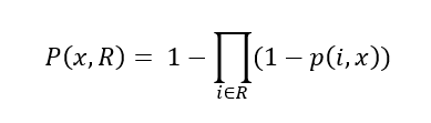
Applying Eq. 1 to the case of the orange ZIP and α we get P(orange, α) = 1 – (1-0.35)(1-0.05)(1-0)(1-0.03) = 0.4. Hence, we can see how the individual trip data is richer and can generate more accurate insights than data at a coarser spatial resolution.
A step forward
While it is true that many businesses do not have access to that level of granularity, it is also true that this type of data is available to many retailers already. For example, many supermarkets and other chains provide their customers with services that rely on GPS data captured by custom apps running on the customers’ smartphones. Moreover, e-commerce has made it common for customers to provide their billing and shipping addresses to retailers, allowing them to exploit these data for spatial analysis even without GPS records.
Suppose the supermarket chain in our example serves the whole area using its two locations, A and B. Table 1 shows a strong preference for customers in the blue and green regions due to distance. However, households in the orange and yellow regions have mixed preferences; some always visit the same location while others visit both with different likelihoods.
Retailers may be interested in influencing groups such as the latter to balance out customer visit distribution utilizing promotions. Indeed, workers at location A, for example, may be overwhelmed, whereas their counterparts at B may have more capacity.
In such a scenario, it makes sense to attract orange and yellow region customers to visit B through some type of promotion. Furthermore, by conducting a geospatial data analysis on the transactions done at A and B by those orange and yellow region customers who visited both, an analyst may find some interesting nuggets such as what pricing and inventory differences drive customers to either location.
Conclusion
Both descriptive analytics and predictive machine learning models can benefit greatly from using geographic information in geospatial data analysis. At Mosaic, we can help you build and implement a custom predictive machine learning model that leverages your geographic data for accuracy and knowledge of segmentation groups. By cleverly using the spatial attributes in the training dataset, we can help you get more robust data analytics and machine learning models for prediction, classification, or clustering.