What is the health state of my industrial equipment? How many hours was I sitting down today? How many customers calling into support are mad, bored, or happy on a given day? These are all questions that can be answered by time-series classification (TSC) models. In the case of Industrial machinery, the machinery health-state can be classified from sensors that are continuously measuring power, temperature, pressure, vibration, etc. Anytime you wish to predict the transient state(s) of something or someone constantly monitored by sensors, TSCs are the right tool. This article will explain some basic concepts of using deep learning models for TSC and finish with a brief discussion of ways to improve the performance to save on cost and speed.
Before discussing time series classification concepts, it is helpful to distinguish them from another similar idea; Time series forecasting. Time-series forecasting is the attempt to predict the next value(s) in the time course. One example of time-series forecasting is predicting the price of a stock upon opening bell the next day. Another example of forecasting is predicting the hourly temperature for the day. In contrast, the goal of TSC is to learn to predict broad transient states and not, typically, future numerical values.
Is deep learning (DL) the appropriate tool for the job?
In time series classification, the goal is to extract distinct temporal patterns related to a particular event (class). Deep learning is particularly suited for extracting high-level patterns from dense large data sets and requires far less pre-processing of input than classical methods. However, DL, though very powerful, comes with a cost. It can be more expensive to develop, requiring GPUs. It also may require a large amount of experienced developer time to produce good results. More traditional time-series classification techniques such as HIVE-COTE are easier and cheaper to develop but often can’t be applied to real-world scenarios. This is because HIVE-COTE and other classical approaches do not tend to scale well. In fact, training time for HIVE-COTE exponentially increases both with a length of the time series and with several input data streams.
To make matters worse, it is impossible to distribute this computing workload across multiple computers, often yielding an impractically long training time. Deep learning approaches, however, scale very well and can achieve high accuracies. Thus, if a time course is relatively short, if there aren’t multiple data streams, or if the temporal data has a natural low-frequency representation, then classical methods may be a better bet. If there are many complex and lengthy time courses, DL may be better.
Some Deep-learning TSC approaches
Some of the first successful deep learning models were image classification models. These models use a series of convolutions (sophisticated ways of combining overlapping blocks of pixels) to learn fine-grained and high-level patterns in images simultaneously. It turns out that this concept can also be applied to time series. Picture unraveling a 2D grid of pixels into a 1D array of pixels, all in a long line. Each pixel is lit up with a specific brightness that is represented as a number. Replace those brightness values with the temperature of your industrial machine, say, and you have a time course. Given the similarities between images classification and TSC, it’s perhaps no surprise that many deep learning TSC models were adapted from image classification models.
How does convolution work for 1D time-courses?
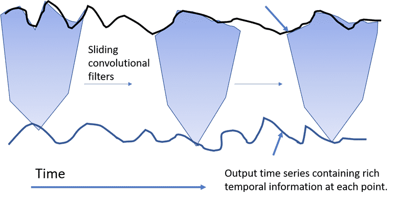
We find it easiest to understand convolutions with a diagram. The figure below demonstrates a 1D convolution on a time series. Sliding filters are applied to a “receptive field” or the length over which the filter is applied. A small receptive field will focus on short-range features, whereas a large receptive field will pick up on patterns over more extended time frames. Typically many layers of these convolutions are performed in series with deeper layers, usually picking up on more and more subtle patterns and edge cases in the data. A final layer is applied to the compressed and feature-rich output of these convolutions to decode them into the most likely class.
Some notable CNN architectures are adapted ResNet and Inception models. If you are interested in the finer details, we will refer you to the original publications (https://arxiv.org/pdf/1909.04939.pdf, https://arxiv.org/abs/1810.07758). In the next section, we will discuss an alternative to CNNs, the Recurrent Neural Network.
Recurrent Neural Nets (RNN) and Long-Short Term Memory (LSTM)
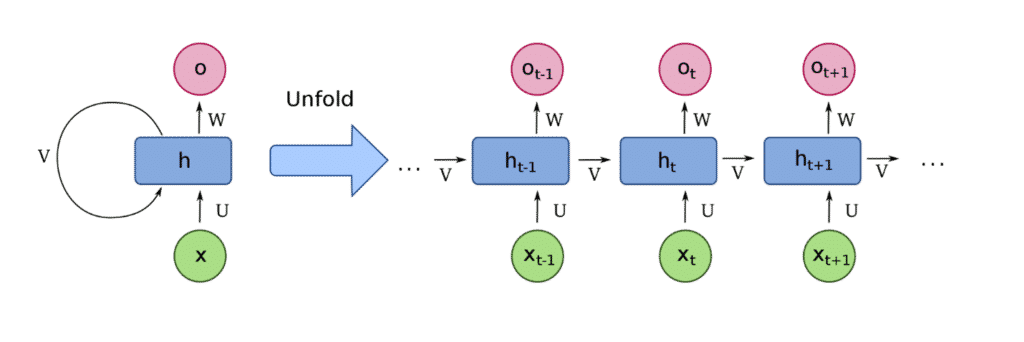
The second main DL architecture element is Recurrent Neural Nets (RNN). RNNs are a broad class of Neural Network motifs that allow outputs from a previous network layer to be passed as the input other (or all) states. (see figure 2) This allows for associating different temporal signals across the entire time series to an arbitrary level. The baked-in sequential nature of RNNs applies to a wide range of applications, including natural language, speech recognition, translation, imagine captioning, and more. Time courses just being one of many applications. The strategy of passing sequential information throughout the network, potentially capturing very long and short-term effects, contrasts with CNNs, which assume that neighboring values in a time course are related. One may think that RNNs would always be better; however, RNNs can carry a significant overhead in computational requirements. If time-series states are expected to be relatively contained within a time window (not influenced by events far in the future or past), then CNN’s can yield more accurate results with fewer computational requirements. One example of this is predicting time sitting down from accelerometer data from a smartwatch. One does not expect the accelerometer data of a sitting person to be significantly influenced by the short walk to stretch their legs minutes previous.
Though it may be more expensive computationally, RNNs may be the best-suited architecture for a particular situation. In this case, there are several different variants of this architecture to choose from; the most common is the LSTM architecture. Though other types of RNNs exist, the LSTM is used by most successful RNN models across a wide range of applications. The reason for LSTM’s popularity is that they solve a significant problem with RNNs. That is, in practice, they have difficulty retaining information about long-term relationships. The real advantage of this architecture over CNNs in the first place! LSTMs solve this problem by a carefully designed series of gates and filters. These gates decide what information from other cells to forget and what information to add. In the final step, a filter is applied to focus future time steps on data that may be more relevant.
Reducing computational requirements
Although DL methods scale well in terms of input time series number and length of the series, they can still require a good deal of computational resources. This is particularly true for training and sometimes true for running predictions. The latter can especially be confirmed if there are many devices on which to run projections.
Several proven strategies exist for reducing the computational requirements of DL models in general. These strategies include increased weight pruning, strategically removing excess hidden layers, weight quantization, and other compression strategies. However, all these strategies come with a catch in that reducing the footprint of a model generally leads to degraded performance.
Another strategy proposed by Chambers and Yoder (https://www.mdpi.com/1424-8220/20/9/2498) proposed a many-to-many TSC architecture. In many TSC arrangements, a sliding window is applied to the input then the model learns (or predicts) on each window generating individual predictions for each time point. A many-to-many approach uses one optimized architecture to learn and predict across a large block of time steps. This leads to more efficient training, with fewer back-propagation steps needed. In addition, they carefully designed the network structure to accommodate longer time series, resulting in better long-range pattern recognition.
Conclusion
If applied correctly, time series classification can be a powerful tool in extracting valuable business and operational insights from dense data streams. We hope this article illuminates some of the broad concepts involved in building a successful TSC model.