Summary
White paper examining how to use MLOps for monitoring production ML code.

Take Our Content to Go
Successfully developing machine learning tools to provide value in a business environment requires much more than algorithmic knowledge and tuning. Machine learning cannot provide value in a vacuum. A simple heuristic deployed in the right place can provide more value than a complex model effectively “mothballed” in an offline setting. At Mosaic Data Science, we take a holistic approach to developing machine learning-enabled solutions. This involves focusing on how the model will ultimately provide value to the business as much or sometimes more than focusing on building the most accurate model.
This focus on delivering and integrating machine learning models is often referred to as MLOps, short for machine learning operations, extending the practice of DevOps in software development. While there are some adjustments that must be made in that extension, we believe that many of the tenets and justifications used in DevOps readily apply to MLOps.
In this white paper, we will outline the development of a machine learning application using MLOps practices. We focus on two main features:
- Continuous model delivery, and
- Production model monitoring and alerting.
We will highlight how these practices reduce operational complexity and time to value, allow for more agile development, and integrate quality assurance into the deployment process. This paper will explore how MLOps provides natural opportunities for fair and ethical machine learning practices that can be implemented, demonstrated, and even audited if necessary.
Business Objectives
For the purposes of this white paper, we simulated a business use case that required an ML application. Our simulated client is a financial services company that provides lending services. Providing this service typically involves reviewing applicants’ financial history and the prospective loan details (e.g., amount, purpose, terms), then using that information to decide on whether to grant loans to each individual applicant. Ultimately, applicants who receive loans may or may not pay the loans back. The objective, of course, is to increase overall profits by reducing instances where the loan is not repaid. The loan approval process is typically manual and based upon human heuristics or other methods.
Business Problem | Increase in Rate of Unpaid Loans
In this demonstration scenario, an unsatisfactory fraction of approved loans are not being repaid, so the lender would like to add a second layer of targeted review of approved but relatively high-risk loans before they are finalized. Having provided lending services for some time, the business has accrued a large data set of loans they have approved, creditor application details, and the ultimate outcome of the loan.
The business wishes to develop a machine learning system to determine which loans are high-risk and thus selected for a secondary review. This system will be used to review all approved loans, and its prediction will be used to automatically approve applications that are predicted to be low risk. All applications that are predicted to be high-risk will undergo a secondary manual review.
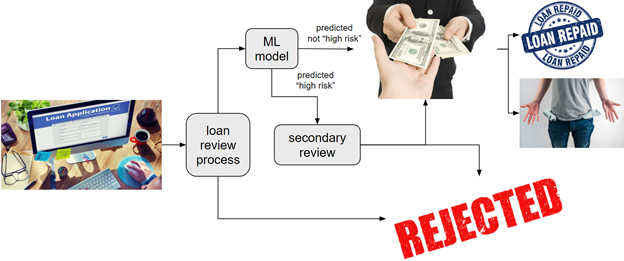
The business anticipates that the secondary review of approved but predicted high-risk loans will be conducted at a relatively high level and will lead to most of those loans being rejected, largely because the marginal cost associated with approving a loan that ends up failing is generally much higher than the marginal cost of failing to approve a loan that would end up being repaid. This situation makes the business much more tolerant of false-positive predictions, i.e., an incorrect classification of a loan as high-risk, than they are of false-negative predictions, i.e., an incorrect classification of a loan as low-risk. In fact, data science efforts on this business case have identified a 5:1 false-negative to false-positive cost ratio for the ML model. This cost ratio enables us to select a low- vs. high-risk threshold on the model’s predicted probability output.
In financial services and other high-stakes settings, issues of fairness and justice are of particular interest in general. These services are under scrutiny by the public and regulators, and the same scrutiny is applied to ML models in this space. The business in the demonstration is keen to develop and deploy a “fair” ML model that reflects its corporate culture and values and will stand up to potential government regulations and associated audits.
Fairness is multifaceted, highly contextual, and use-case specific. It may not be possible to simultaneously accomplish all relevant notions of fairness. Furthermore, increases in fairness may be offset by decreases in predictive accuracy or other quality metrics, so priorities must be evaluated, and value judgments are typically required. Across the board, the fairness of an ML model is not proven, but rather constantly measured, with scrutiny and adjustments provided based on measurement results. We will demonstrate how this constant measurement can naturally be built into an MLOps pipeline.
Ethical ML Model Frameworks
After reviewing the business problem and proposed solution, we recommended that the business evaluate the model using the Equal Opportunity framework of fairness. This popular and well-studied notion of fairness focuses on assessing whether the model is less accurate when making predictions for any protected sub-group than for other sub-groups. For this assessment, Mosaic recommended using the false-positive rate as the key error metric. This is because the positive prediction (a loan classified as high-risk) is punitive to the applicant. If the model incorrectly classifies an applicant’s loan as high-risk, it will likely result in an unfair rejection of the applicant’s loan. In the demonstration scenario, the business is mostly concerned with being fair with respect to applicant ethnicity.
To evaluate our loan approval ML model using the Equal Opportunity framework of fairness, we need to compare the false-positive rates for each ethnic group. We do so by calculating the absolute differences between all the groups’ false-positive rates. If the largest of those differences is too far from zero, then the model fails to achieve Equal Opportunity fairness, a situation that merits further attention and potential intervention.
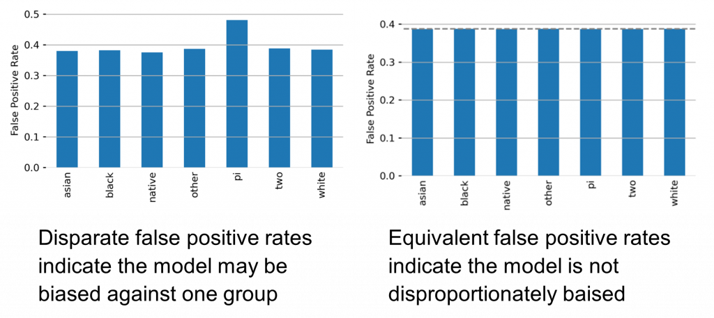
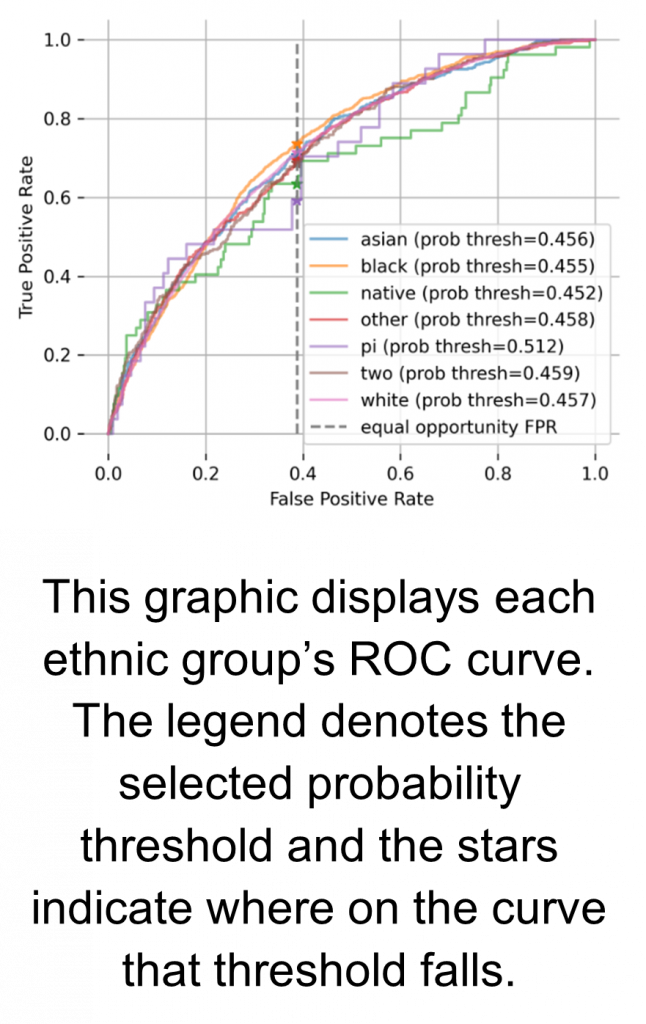
Fortunately, there is a relatively straightforward way to adjust a trained ML model to ensure that it satisfies the Equal Opportunity notion of fairness. We can ensure that each group achieves the same false-positive rate by adjusting the low- vs. high-risk predicted probability threshold per ethnic group to hit the specified rate. For instance, if loans from a certain ethnic group are being flagged as high-risk more often than loans from other ethnic groups, we can change the probability threshold in the model for the particular ethnic group, adjusting it until we reach equivalent false-positive rates. We then search over candidate false-positive rates to find the one that minimizes the 5:1 cost ratio described earlier. This approach maximizes the lender’s profits within a fairness constraint. The figure below demonstrates how setting group-based probability thresholds can ensure uniform false-positive rates.
At this point, we’ve established a notion of fairness, a way to measure it, requirements for what measurements are acceptable, and a way to address unacceptable measurements. But how do we make sure the measurements are consistently run for every model? What is the process for reviewing these measurements when the fairness of a model comes into question? How do we prevent a model that does not meet these requirements from adversely impacting our client or their prospective clients (the loan applicants)? How do we know whether a model continues to meet these requirements after it’s been deployed? These are all questions MLOps can help answer. Next, we will explore how continuous model delivery can integrate fairness testing and requirements into the deployment pipeline, and how production model monitoring can alert users about potential issues in a deployed model.
Continuous Model Delivery
Continuous model delivery is the machine learning equivalent of continuous integration and delivery (often referred to as CICD). CICD is the practice of automating all the operational tasks required to build and deploy an application. It treats the deployment of the application as a part of the application, including automation of the application deployment in the source code, right next to the core application logic. Continuous model delivery includes everything from the environment configuration (e.g., downloading and installing python packages) to launching the application itself.
Furthermore, this approach eliminates the gap between development and operations by using source code as the trigger for the deployment. If any test fails, so does the pipeline, preventing flawed code or flawed models from reaching the users. As soon as a code change is published, the automated build process begins. This includes everything from setting up the servers and running the application to testing and QA, making sure that every change is tested.
This coupling of development and operations encourages frequent releases, promotes traceability, and reduces risk of operational errors. The trade-off here is between the complexity of developing the application and the complexity of operating it. While it may be more complex to build this automation of operations into the application, it is easy to isolate end users from that complexity and the “extra” work in setting up automation will ultimately produce an application that is both higher quality and easier to maintain over the long term.
As applied to machine learning applications, continuous model delivery involves automating the training, evaluation, and deployment of the model. The model is the crucial component of the machine learning application and with it comes additional complications that aren’t seen in typical software applications. While the performance of typical software applications only depends on code, ML applications depend on both code and data.
ML applications are more reliant on testing than other applications. If you’re a data scientist, you know by experience that just as much, if not more, of your time is spent evaluating your model as training it. Another common scenario is when a trained model may be operationally fine, passing all unit tests, but may not meet statistical quality expectations concerning accuracy, fairness, or other performance metrics, which are measured on large data sets and thus are highly dependent on the distribution of the input data.
Data scientists invest so much time into ensuring the quality of the model because model quality is crucial to the success of the application. Integrating the often-complex quality testing into the automated application delivery makes a lot of sense in a machine learning context. Implementing the continuous model delivery framework provides an easy-to-manage “paper” trail from a running application back to training and evaluation metrics and ultimately back to code, data, and parameters used for training.
Pipeline Implementation
When implementing this kind of system, we believe that it is crucial to plumb the system through as soon as there is consensus that a model should be deployed, even if the model initially deployed is just a placeholder or heuristic. The sooner you have the deployment automated, the less time you need to spend on manual deployment. More important, though, this approach reduces time to value. Getting the ML application deployed earlier allows stakeholders of other systems that may begin to rely on your model to start figuring out how their application will work with your model outputs. This enables earlier feedback and a greater likelihood of buy-in from application users.
For the business case we’re exploring, we will be deploying the lending risk prediction model as an HTTP API implemented in Flask. Our model is trained and evaluated on a designated VM. This is crucial to the use case because sometimes models must be trained on specialized hardware, such as GPUs. We are using an additional tool called MLflow to help with model management. MLflow acts as a broker for the models, helping manage different versions of models, record the performance metrics they produced during training, and provide traceability back to the parameters and code that were used to train them. We use a Jenkins pipeline to orchestrate all the steps that are required to train, evaluate, and deploy the model.
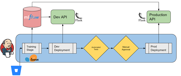
The Jenkins pipeline automates all the operational tasks. The pipeline is set up as a script of steps that need to be performed to deploy the model. Jenkins can both run these pipelines and keep track of their progress and results. Jenkins monitors a branch of the source control repository, and when a change is committed to that branch, a pipeline run is launched. A data scientist only has to commit the code to the production branch and allow the automation to do the rest.
The pipeline run proceeds in multiple stages. The first is to train the model. Jenkins connects to the training server via SSH and receives the code that was updated. It prepares the environment by installing new packages managed in the conda environment file. Then, using command line scripts, the pipeline runs the training and evaluation developed by the data scientist. In this case, the training code has been instrumented with the MLflow API to log the parameters and evaluation metrics of each run to the MLflow server. Artifacts of the model training run, most importantly the trained model itself, are archived in a cloud storage MLflow artifact store where they can be easily accessed for further deployment or evaluation.
The next stage is to deploy the model to the development environment. The Jenkins pipeline proceeds to connect to this server via SSH, download the model service code and prepare the python environment. At this point, it runs the model service API code. The model service code is configured to connect the MLflow server and pull down the model. MLflow in this situation is analogous to a PyPi server, where you can download different versions of a python package and install them; in this case a model is installed instead of a package.
At this point, the model has been fully deployed in an isolated development environment. This allows us to get a full preview of what the model would look like in production. But before we go there, it is time to test. Now we perform our unit tests, integration tests, and performance requirement tests. Integration tests go a step further than testing an application itself in that they test how an application interacts with others in the system, essentially making sure your application integrates with others before it hits prime time (the production environment).
The model-training run initiated by Jenkins will evaluate the model by asking it to make predictions on a “test” data set that was not used during training. Results of this evaluation are logged in MLflow, and we can simply check out the metrics using the MLflow API and compare them to our requirements. This fits really nicely into a unit test framework such as xUnit. This automated testing stage is our opportunity to enforce the requirements that an application must meet before it can be deployed to our users. This includes implementing the Equal Opportunity fairness requirement.
If the application passess the automated tests, there is one last stage before the model is deployed to production: a manual approval stage. In this stage, Jenkins automatically emails specified data scientists and business leaders and waits for them to approve the deployment to production. At this stage, the approvers have everything they should need to make their decision. All the training details are recorded in MLflow, the test results have been published, and the approvers can access and interrogate a running instance of the model service. At Mosaic, we believe it is important to keep a human in the loop for this final approval stage.
After approval, the pipeline proceeds to deploy the application to production. This stage is essentially the same as model deployment to the development environment except that the configuration is set so that the application is deployed into the user-facing environment, where it can be used during business operations.
To recap, we have automated the deployment process, which (1) ensures consistent and automatic reviews of the ML application that will ultimately reach business users and (2) frees up data scientists to spend more time on innovative machine learning solutions and less on delivery. But what happens once the application is in production? Just as much can go wrong in production as deployment…can MLOps help with this?
Production Monitoring and Alerting
One of the fundamental assumptions one makes when developing and deploying machine learning applications is that the data that is produced in the production environment is similar to the training data and the environment that produced it. This is an unfortunately brittle assumption. Events can have large and complex impacts on data-producing systems that may ultimately degrade the performance of machine learning models. For example, you might be able to imagine how a global pandemic could break some assumptions a model inherited from its training data. An ML model itself might start changing the data-producing system when it gets deployed! Unfortunately, while MLOps itself doesn’t have any good answers for how to address these issues, it can help proactively detect them.
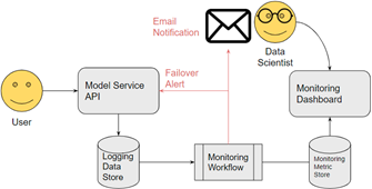
The solution we propose is called production model monitoring and alerting. Monitoring and Alerting is a DevOps practice of instrumenting applications to provide a transparent log of everything the application does and monitoring this log for any activity that the developers would not expect to see. We see this as a useful tool for machine learning applications as well.
Data Drift describes the phenomenon when data the model is seeing becomes different from data that it was trained on. We see data drift detection as a key use case for model monitoring and alerting. We essentially instrument the model service to log all of its predictions and inputs. Then on a regular basis, we perform statistical tests to compare the latest data to the data the model was trained on. If any changes are detected, the system will alert relevant parties (such as an on-call data scientist) and trigger the model service itself to begin performing failover processing.
Regardless of the metric, the models are initially trained with only a random subset of historical data and validated against a separate subset of data. This process of cross validation is repeated multiple times to ensure that the algorithm and parameter setting selections are repeatable and not biased by the chance selection of training sets. The final model is trained with all the relevant historical data (egregious outliers are removed).
Dashboard Development
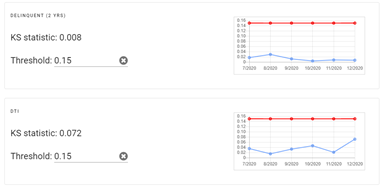
The model dashboard is a persistent way to visualize the results of the monitoring workflow. The dashboard is split into three panels. The first panel focuses on traditional monitoring metrics such as the number of requests the service has received, the number of errors it produced, and the number of positive predictions that were returned. This panel provides a high-level overview of the operations and performance of the server.

The next panel shows the metrics for testing drift in the inputs to the model. The goal of this test is to determine whether the features that are being scored in production follow the same distribution that they did in the training data. The nature of the feature determines what test should be used. The Kolmogorov-Smirnov Test is used for continuous/numeric features. Kullback-Leibler divergence is used for discrete/categorical features. These metrics are compared to a predefined threshold for testing.
The last panel focuses on the output of the model. In our business case, we won’t know how many loans are repaid until the terms of the loans are complete, so we are unable to directly monitor the predictive accuracy of the model and the fairness test we developed. However, there are some closely related quantities that we can monitor to give us a good idea about our metrics of interest. We can perform a test to see if the proportion of positive predictions in the production data is the same as the proportion of positive predictions in the training data. We do so by estimating a confidence interval for the proportion of positive predictions in the training set assuming a sample of the same size as the production data requests. We can perform this test per the ethnic group of the loan applicants. If we see a change in the positive prediction proportion, it may be evidence that the false positive rates have changed as well.

Conclusion
This white paper used a simulated business case to demonstrate how MLOps can support machine learning solutions with built-in quality assurance and fairness testing. There are many other use cases and ethical frameworks that can be supported by MLOps.
At Mosaic Data Science, we build machine learning solutions on two foundational pillars. First, we take a design-oriented approach to frame the problem and develop the right machine learning solution to address it. Second, we take great care in integrating the machine learning solution into the business process with an eye for sustainability and maintainability.
We believe that building machine learning solutions requires focusing on operations and delivery as much as the development of the algorithm itself. Our holistic approach differentiates us from others in the market because we focus on developing custom applications that fit your ecosystem rather than trying to shoehorn prebuilt solutions that ultimately don’t integrate into your workflow. If you’re interested in seeing a live demonstration of the systems described in this white paper and further exploring how we can help with your business case, please contact us.


